Bollinger Bands Backtest Demo
Explore how to use Exchange Outpost to evaluate a trading strategy by backtesting it on multiple symbols simultaneously.
Variance is a statistical measurement of the spread between numbers in a data set. In finance, variance is used to measure the volatility of an asset's price over time. A high variance indicates that the price of the asset has been more volatile, while a low variance indicates that the price has been more stable.
Low Variance (σ² = 0.04)
Mean: $100.15 | Stable price movement
High Variance (σ² = 104.80)
Mean: $100.00 | Volatile price movement
Key Insight: The dashed line represents the mean price. Notice how the low variance data stays close to the mean, while the high variance data spreads much further from it. This spread (variance) is what Bollinger Bands use to create their upper and lower boundaries.
In financial markets, price movements often follow patterns similar to a normal distribution around a moving average. This statistical behavior is the foundation of many trading strategies, including Bollinger Bands.
The Normal Distribution (Bell Curve) tells us that:
- 68% of price movements stay within 1 standard deviation of the mean
- 95% of price movements stay within 2 standard deviations of the mean
- 99.7% of price movements stay within 3 standard deviations of the mean
68% of prices fall within ±1σ of the mean
68% of prices fall within ±1σ of the mean
95% of prices fall within ±2σ of the mean
Statistical Foundation: In a normal distribution, approximately 95% of all values fall within 2 standard deviations of the mean. This means that when a price moves beyond the ±2σ bands, it's statistically "unusual" and likely to revert back toward the mean. This is the mathematical basis for Bollinger Bands trading signals.
When a price moves beyond 2 standard deviations (the outer Bollinger Bands), it's statistically unusual - happening only about 5% of the time. This rarity suggests the price is likely to revert back toward the mean, making it an attractive entry point for mean reversion trades.
Trading Insight: The mathematical probability that prices will stay within the bands most of the time (95%) is what makes Bollinger Bands effective. When prices do break out beyond 2σ, the statistical tendency is for them to "snap back" toward the moving average.
Bollinger Bands are a type of statistical chart characterizing the prices and volatility over time of a financial instrument or commodity, using a formulaic method propounded by John Bollinger in the 1980s. Financial traders employ these charts as a methodical tool to inform trading decisions, control automated trading systems, or as a component of technical analysis.
Bollinger Bands consist of three lines:
- A simple moving average (SMA) in the middle.
- An upper band, which is the SMA plus a certain number of standard deviations (typically 2).
- A lower band, which is the SMA minus the same number of standard deviations.
Simple Moving Average - the baseline trend
SMA ± 2 standard deviations - volatility boundaries
Actual price movement relative to the bands
Trading Signals: When price touches the upper band (day 9, 11), it may indicate an overbought condition. When price touches the lower band (day 10), it may indicate an oversold condition. Notice how the bands expand during volatile periods and contract during stable periods.
The bands expand and contract based on market volatility. When the market is more volatile, the bands widen, and when the market is less volatile, the bands contract.
When the price of the asset moves closer to the upper band, it is considered overbought, and when it moves closer to the lower band, it is considered oversold. Traders often use Bollinger Bands to identify potential buy and sell signals.
The basic idea behind the strategy is to buy when the price of the asset moves below the lower band and sell when it moves above the upper band.
The strategy can be implemented in the following steps:
- Calculate the Bollinger Bands for the asset using a specified period and standard deviation.
- Monitor the price of the asset and look for buy and sell signals.
- When the price moves below the lower band, it is considered a buy signal.
- When the price moves above the upper band, it is considered a sell signal.
- Exit the position when the price moves back to the middle band (SMA).
Risk Management: Most traders prefer to use a target profit and stop loss to manage risk. A common approach is to set a target profit at a certain percentage above the entry price and a stop loss at a certain percentage below the entry price.
Mean Reversion Strategy: This strategy assumes that price movements that reach the outer bands are temporary extremes and that prices will tend to revert back toward the mean (middle band). Entry occurs at the bands, and exit occurs when price returns to the SMA.
This comprehensive example shows how the Bollinger Bands strategy would perform over 30 trading days with realistic price movements, volume data, and clear buy/sell signals marked.
Buy Signals (5)
Sell Signals (3)
Strategy Performance Analysis
Note: This demonstrates signal identification only. A complete backtest would include position sizing, transaction costs, and risk management rules.
Key Observations:
- Buy signals occur when price touches or breaks below the lower band
- Sell signals occur when price touches or breaks above the upper band
- Higher volume often coincides with band touches, confirming signals
- The bands expand during volatile periods and contract during consolidation
Strategy Rules Applied:
- Entry: Price touches outer band (buy at lower, sell at upper)
- Exit: Price returns to middle band (SMA)
- Mean reversion: Assumes price will return toward average
- Volume confirmation: Higher volume strengthens signals
Let's see how we can backtest the Bollinger Bands strategy using Exchange Outpost. We're going to write the backtesting code in Rust, which will grant us the best performance and flexibility. We're going to use the ta library to calculate the Bollinger Bands.
1. Define Basic Types
Loading...2. Implement the Run Function
Loading...3. Load Data and Parameters with Validation
Loading...4. Initialize Backtest Data
The data for the running backtest will be stored in these 2 variables:
Loading...- 1.
trades: a vector that will store all the closed trades. - 2.
open_trade: an optional variable that will store the currently open trade, if any.
5. Initialize Bollinger Bands
Loading...6. Execute the Backtest
Process remaining candles for the backtest with stop-loss and take-profit logic:
Loading...7. Cleanup Remaining Positions
We still need to cleanup any remaining open position at the end of the backtest:
Loading...8. Calculate Final Results
Finally we can calculate the total profit and return the result with symbol and exchange information:
Loading...Enhanced Strategy with Risk Management: This implementation includes stop-loss (SL) and take-profit (TP) functionality for better risk management. The strategy opens short positions when price exceeds the upper band and long positions when price drops below the lower band, with automatic position closure based on the configured risk parameters. Most traders prefer to use a target profit and stop loss to manage risk.
Exchange Outpost Advantage: With Exchange Outpost, you can run this backtesting code across multiple symbols simultaneously with serverless scaling and instant access to historical market data.
Now it's time to use the function we created to run a backtest. Let's start by backtesting the strategy on BTCUSDT perpetual futures on a timeframe of 1m from 1st of August 2025 to 1st of September 2025.
Getting Started: Push your code to GitHub using theRust function templatewhich provides automated CI to build your code.
Backtest Results Across Different Assets
BTCUSDT Perpetual Futures
+87.04 USDTLoading...Trades have been omitted for brevity - This means the strategy made a profit of 87.04 USDT in one month when trading BTC perpetual futures with 1000 USD, not bad for such a simple strategy!
ETHUSDT Perpetual Futures
-54.79 USDTLoading...Poor performance on Ethereum perpetual futures
BNBUSDT Perpetual Futures
+66.30 USDTLoading...Good performance on BNB perpetual futures
From these initial backtest results, we can see that our simple Bollinger Band strategy performs differently across various cryptocurrency perpetual futures:
BTCUSDT
Excellent performance
ETHUSDT
Poor performance
BNBUSDT
Good performance
Key Insights
- • Strategy performance varies significantly between different cryptocurrencies
- • The strategy works well on the major cryptocurrencies like BTC and BNB
- • ETH struggles with this strategy in this particular timeframe
- • This demonstrates the importance of testing strategies across multiple assets
To get a more comprehensive view of our strategy's performance, we used a Python script to run this backtest across 10 major cryptocurrency symbols over multiple time periods and parameter configurations. This comprehensive analysis provides statistical insights into which assets and market conditions are most favorable for the Bollinger Bands mean reversion strategy.
Benefits of Multi-Asset Testing
- • Identify which asset classes work best with your strategy
- • Understand correlation between market conditions and strategy performance
- • Build robust portfolios by diversifying across multiple profitable assets
- • Discover unexpected opportunities in lesser-known trading pairs
Let's use Python to run our Bollinger Bands strategy across multiple symbols and time periods. This will help us identify which assets and market conditions are most suitable for our strategy.
1. Setup API Configuration
First, configure your Exchange Outpost API credentials and define your testing parameters:
Loading...2. Define Backtest Functions
Create helper functions to start backtests and retrieve results:
Loading...3. Configure Test Symbols and Parameters
Define which symbols to test and what parameter sets to use:
Loading...Parameter Variation: Testing multiple parameter sets helps identify optimal configurations for different market conditions and trading pairs.
4. Generate Time Periods
Create multiple time windows to test strategy robustness:
Loading...5. Execute Batch Backtests
Build and submit all backtest combinations:
Loading...Parallel Execution: Exchange Outpost automatically parallelizes these backtests across its serverless infrastructure, dramatically reducing total execution time.
6. Analyze Results
Process and analyze the backtest results using pandas:
Loading...Real-World Testing Results
Running this comprehensive test across 10 symbols, 18 time periods, and 5 parameter sets generates 900 individual backtests. With Exchange Outpost's serverless architecture, all 900 tests complete in minutes rather than hours.
Key Findings from Multi-Symbol Analysis
- • Strategy performance varies significantly: Some symbols show consistent profitability while others consistently lose money with the same parameters
- • Parameter sensitivity: Different parameter combinations work better for different market conditions and volatility levels
- • Time period matters: The same strategy can be profitable in some time windows and unprofitable in others, highlighting the importance of testing across multiple periods
- • Diversification benefits: By identifying multiple profitable symbols, you can build a diversified portfolio that reduces overall risk
7. Group Results by Parameter Set
To analyze how different parameters affect strategy performance, group the results by parameter configuration:
Loading...This code extracts unique parameter sets, filters the dataframe for each set, and sorts them by total profitability.
8. Analyze Each Parameter Set
Generate comprehensive statistics for each parameter configuration:
Loading...This iterates through each parameter set and displays:
- • Overall statistics (total profit, win rate, number of trades)
- • Top performing symbols for that parameter set
- • Symbol-wise win rates and profitability
View calculate_and_print_param_stats() implementation
Loading...Results with Default Parameters
Below are the comprehensive analysis results achieved with the default parameter set (Period: 20, Multiplier: 2, Stop Loss: 2%, Take Profit: 4%). These results demonstrate the strategy's performance across all 10 symbols and 18 time periods.
================================================================================
BOLLINGER BANDS STRATEGY - COMPREHENSIVE ANALYSIS BY PARAMETER SET
================================================================================

================================================================================
PARAMETER SET P20_M2_SL0.02_TP0.04
================================================================================
Period: 20, Multiplier: 2, SL: 0.02, TP: 0.04

📊 OVERALL STATISTICS
--------------------------------------------------------------------------------
Total backtests run: 180
Total profit across all backtests: $5,687.59
Average profit per backtest: $31.60
Median profit per backtest: $25.87
Win rate (profitable backtests): 54.44%
Total trades executed: 35,155
Average trades per backtest: 195.31

🏆 TOP PERFORMERS
--------------------------------------------------------------------------------
Best performing symbols (total profit):
  1. LINKUSDT: $3,291.36
  2. SOLUSDT: $3,266.20
  3. ADAUSDT: $3,248.52

📈 SYMBOL-WISE WIN RATES
--------------------------------------------------------------------------------
  ADAUSDT: 72.2% win rate | Total profit: $3,248.52
  LINKUSDT: 66.7% win rate | Total profit: $3,291.36
  SOLUSDT: 61.1% win rate | Total profit: $3,266.20
  ETHUSDT: 61.1% win rate | Total profit: $426.57
  DOGEUSDT: 55.6% win rate | Total profit: $-277.40
  DOTUSDT: 50.0% win rate | Total profit: $-1,410.72
  XRPUSDT: 50.0% win rate | Total profit: $184.09
  BNBUSDT: 44.4% win rate | Total profit: $-1,084.12
  BTCUSDT: 44.4% win rate | Total profit: $522.43
  AVAXUSDT: 38.9% win rate | Total profit: $-2,479.34

--------------------------------------------------------------------------------
Key Insights
- Overall Performance: The strategy achieved a total profit of $5,687.59 across 180 backtests with a 54.44% win rate
- Best Performers: LINKUSDT, SOLUSDT, and ADAUSDT showed exceptional performance with profits exceeding $3,200 each
- Win Rate Leaders: ADAUSDT led with a 72.2% win rate, followed by LINKUSDT at 66.7%
- Trading Volume: 35,155 total trades were executed, averaging ~195 trades per backtest period
- Volatility Impact: Higher volatility assets like AVAXUSDT showed negative performance, suggesting the need for parameter optimization
Parameter Set Comparison
To visualize how the default parameters performed across different symbols and time periods, we created a profit heatmap. This visualization helps identify patterns in profitability over time and across different cryptocurrency pairs.
Creating the Profit Heatmap
Using the filtered dataframe with default parameters, we can create a comprehensive heatmap that shows profit distribution across all symbols and time periods:
Loading...Generated Heatmap Visualization
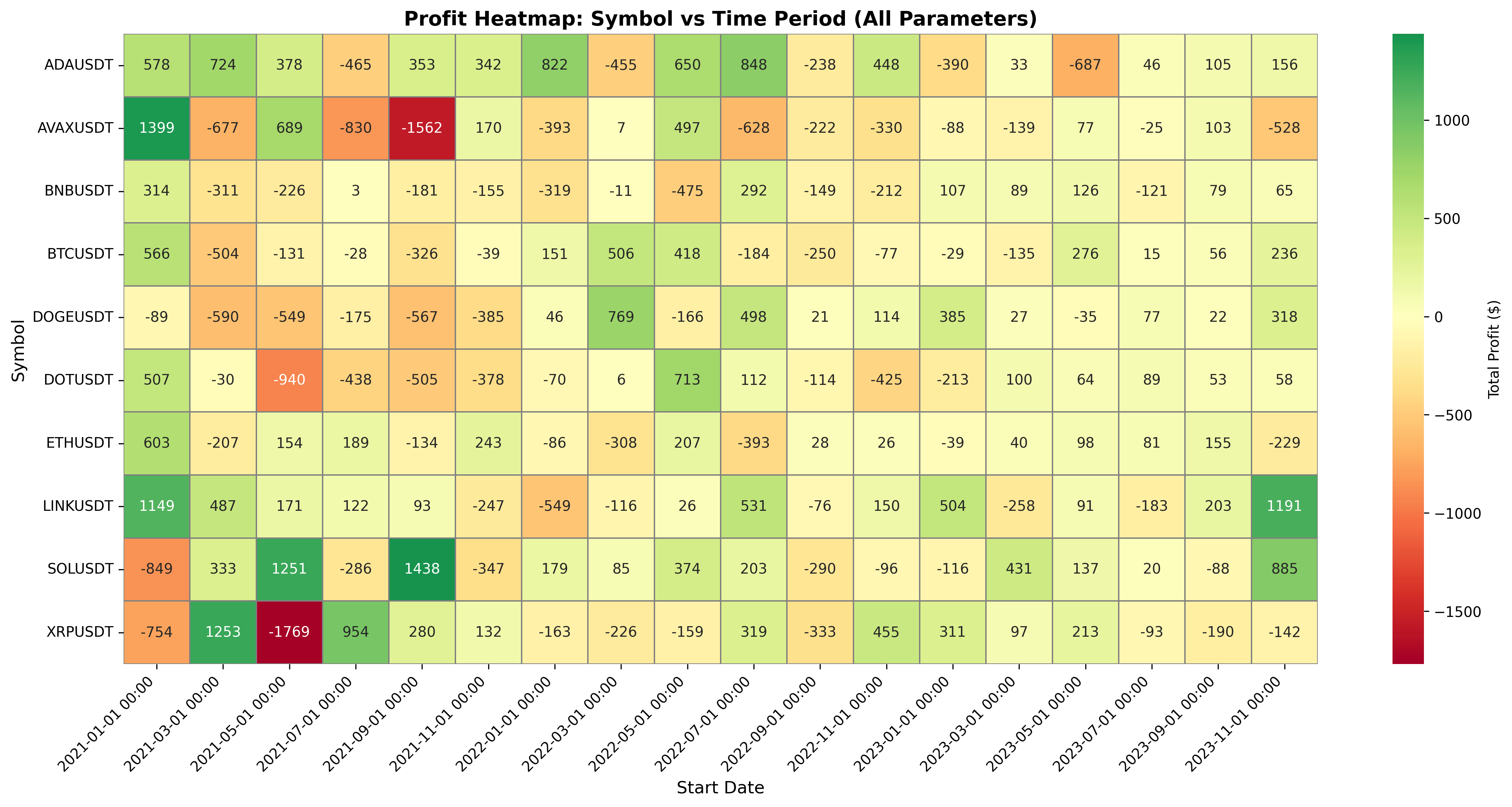
Profit heatmap visualization showing the default parameter set performance across all symbols and time periods
Heatmap Insights
- Color Coding: The heatmap uses a Red-Yellow-Green color scheme where green indicates profitable periods, red shows losses, and yellow represents near-breakeven performance
- Temporal Patterns: You can identify which time periods were generally more profitable across multiple symbols, revealing market-wide trends
- Symbol Performance: Rows show how individual symbols performed across all time periods, making it easy to spot consistently profitable or unprofitable assets
- Hot Spots: Dark green cells highlight the most profitable symbol-period combinations, which could be investigated further for pattern analysis
- Risk Assessment: Clusters of red cells indicate periods or symbols where the strategy struggled, helping identify conditions to avoid or parameters to adjust
Conclusion & Key Takeaways
Scale & Performance
This comprehensive backtest demonstrates the power of Exchange Outpost's serverless financial functions. By executing 900 backtests across 10 cryptocurrency pairs, 18 time periods, and 5 parameter configurations, we processed approximately 79.2 million data pointsin just ~1 minute.
Strategy Performance
- ✓54.44% win rate with default parameters
- ✓Total profit of $5,687.59
- ✓35,155 trades executed successfully
Top Performers
- 🥇 LINKUSDT$3,291.36
- 🥈 SOLUSDT$3,266.20
- 🥉 ADAUSDT$3,248.52
Key Insights
- •ADAUSDT led with a 72.2% win rate, demonstrating asset-specific performance variations
- •Temporal patterns revealed market condition dependencies visible in the heatmap analysis
- •High volatility assets like AVAXUSDT show potential for parameter optimization
🚀 The Exchange Outpost Advantage
This demo showcases how Exchange Outpost enables traders and researchers to rapidly test and iterate on trading strategies at scale. Whether developing new strategies, optimizing existing ones, or conducting market research, our serverless architecture provides the computational power and flexibility for comprehensive financial analysis.
Ready to Build Your Own Strategy?
Start backtesting your trading strategies with Exchange Outpost's serverless financial functions.